Using R

To use R you’ll need to learn how to write some basic code. Fortunately R is a comparatively simple programming language to learn, it has:
- a simple and tolerant syntax (this is like the ‘grammar’ of programming languages),
- extensive help resources written for people without programming skills,
- thousands of extension packages that make your analysis easier,
- a friendly and supportive community of R users!
You can code! If you’ve used a calculator you’ve already written code, code is simply instructions made for a computer (like an equation for a calculator).
R as a calculator
Just like a calculator, R can be used to perform basic arithmetic (and a whole lot more!). Try out the following examples:
Using functions
R is a functional programming language, which means that it primarily uses functions to complete tasks. A function allows you to do much more than basic arithmetic, they can do almost anything!
Example:
To take the natural logarithm of 1, you would write:
In this example:
logis the name of the logarithm function(1)is the input to the function
You can look at the help file for any R function using ? or help(), try looking at the documentation for log:
In this documentation (scroll down to Usage) you’ll see that the log() function can accept 2 inputs: log(x, base = exp(1)).
By default the logarithm’s base is exp(1) or \(e\) (giving the natural logarithm), but you can change this by specifying a different base. Try changing the logarithm’s base to 10:
Hint
The log() function can take an optional base parameter to specify the logarithm’s base. By default, it uses the natural logarithm (base e), but if you want to compute the logarithm with base 10, you can specify it as follows.
log(1, base = 10)Syntax
Syntax is the grammatical rules of a programming language, and while R has a flexible syntax it does have rules.
Just like on a calculator, it doesn’t make sense to ask what 3 */ 5 is. So what does R do? Try it!
R returns a ‘syntax error’ because it didn’t expect a division (/) to occur immediately after multiplication (*). While errors can be intimidating, they’re really trying to help. A syntax error in R starts with “unexpected” and then describes the part of your code which violates the syntax rules.
Syntax errors are commonly from mismatched quotes ('...', "...") or brackets ((...), {...}), and can be tricky to fix. We’ll learn more about fixing errors in the next lesson about troubleshooting.
Code comments
One way to make your code easier to understand is to add code comments. Any code after # will be completely ignored by R, allowing you to write helpful notes about what your code is doing. This is especially useful when sharing your code with others (or your future self)!
Add a code comment that explains what this code is doing:
Hint
To include a comment in your code, start with the # symbol followed by your explanatory text. Comments help explain what the code is doing or why certain decisions were made.
# This calculates the exponential of 1, returning Euler's number (e)
exp(1)
The pipe, |>
A lot of functions in R (especially tidyverse functions) are designed to be chained together using |> (the pipe). The pipe simply takes the result of the code on the left, and inserts it into the function on the right.
Example:
Writing long chains of code with the pipe makes your code easier to read and can be documented with comments. The equivalent code without the pipe is mean(exp(rnorm(1000))), which you read from the innermost set of brackets outwards. With the pipe, we say rnorm(1000) is ‘piped’ into the exp() function giving exp(rnorm(1000)) which is then piped into the mean() function.
The magrittr pipe,
%>%
You might encounter a similar looking magrittr pipe (%>%) in examples online. It is included in the magrittr package, and behaves very similarly to the native pipe.
The native pipe (|>) was added to R in version 4.1.0 directly into R’s syntax, and is recommended for use with new code.
Objects
Objects are used to store data in R, which can be recalled later for use in other code.
You can create an object with the assignment operator <-. You can also use =, but we recommend sticking to <- since = is also used for named function inputs.
If successful, it will look like nothing has happened because objects are created silently (no output messages). In RStudio, you will be able to see e added to your environment pane (top-right) with the value 2.7182818.
This object can be reused in other code, for example try computing the logarithm of e:
Hint
To compute the natural logarithm of Euler’s number ( e ), re-use the e variable you have previously defined. Recall that ( e ) can be represented by exp(1) which you’ll use as follows:
e <- exp(1)
log(e)
Object naming
A clear and descriptive object name is an important for your code to be readable, maintainable, and less error-prone.
There are two main styles commonly used in R:
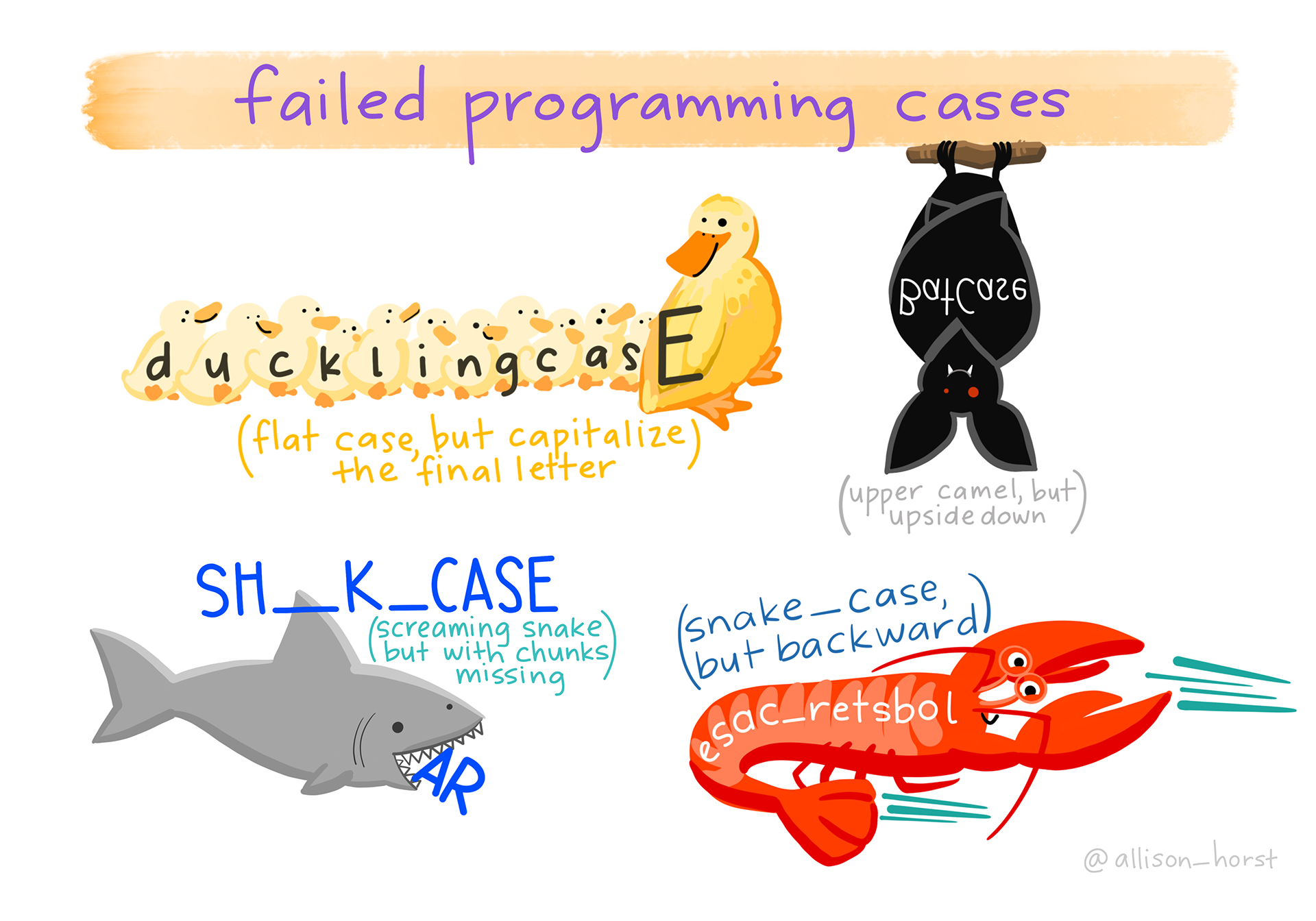
You can use any object name you like (R doesn’t care), but we recommend that you:
Be concise and descriptive
No-one likes to write out a
really_long_object_name, however a clearly described variable is far better thanxandy.Spell out all relevant details, for example
temperature_celsiusis better thantemperatureortemp(which can be confused for temporary).Be consistent
Choose a naming convention (we recommend
snake_case) and stick to it.Avoid existing names
Try not to use names that are already used in R, especially not reserved words like
TRUEandFALSE.Common conflicting names include
dtanddf, which are the densities of t and F distributions (not abbreviations ofdataordata.frame).Use underscores only, no other special characters
A lot of special characters (e.g.
$,@,!,.,#) have special meanings in R, and should not be used.Fun fact: Until R v2.0.0 (October 2004), underscore was the assignment operator!
Data types
Each object in R has a type, here are some commonly used data types:
Numeric:
42,3.14With sub-types:
- Integer:
42L(without decimals, theLindicates integer) - Double:
3.14(with decimals)
- Integer:
Character:
"startr"Logical:
TRUEandFALSEDate and Time:
Sys.Date()andSys.time()
R also supports some special data types commonly used in statistics and data analysis:
Missing values:
NAEach data type can contain NA (not available) to indicate unknown values.
Complex:
1 + 2iComplex numbers consist of real and imaginary parts.
You can check the data type of a variable with the class() function, and check if an object is a particular type with is.*() (for example is.numeric() and is.logical()).
Mixing data types
R automatically converts between data types for you as needed, generally this is helpful and works well but it can sometimes be surprising.
Experiment with combining different types of data mathematically, and try to reason why you get each result.
Many of these mixed data type operations convert one type into another, in the above example:
1L + 3.5: the integer (1L) became a double (1.0)TRUE + 3: the logical (TRUE) became numeric/double (1.0)
You can explicitly convert an object into a different type using as.*() functions (for example as.numeric() and as.character()).
Vectors, matrices and arrays
These objects contain multiple values of the same data type, organised into 1D vectors, 2D matrices or higher dimensional arrays.
Vectors
A vector can contain multiple (0 or more) values of the same data type. Vectors are used extensively in R since datasets typically contain more than one observation! A singular value (usually a ‘scalar’ in other languages) is handled as a length 1 vector, so all of the previous examples have used R vectors.
The c() function (the combine function) is used to combine multiple vectors together.
You can also generate sequences with seq(), or simply with from:to for integer sequences.
Some other useful vector functions include:
Mathematical Summaries:
sum(): Calculate the total of all elements.
mean(): Compute the average value.any(): Check if any element is TRUE.
all(): Check if all elements are TRUE.
min(): Find the minimum value.
max(): Find the maximum value.
median(): Compute the middle value.
quantile(): Compute specified quantiles.
sd(): Calculate the standard deviation.
var(): Compute the variance.
prod(): Calculate the product of all elements.
Cumulative maths:
cumsum(): Compute the cumulative sum of elements.
cumprod(): Compute the cumulative product of elements.
diff(): Calculate the differences between consecutive elements.
Vector Manipulation :
rep(): Replicate elements in the vector.sort(): Sort elements in ascending or descending order.
rev(): Reverse the order of elements.
length(): Get the number of elements in the vector.table(): Create a frequency table of elements.
Set Operations:
union(): Combine elements from two vectors, removing duplicates.
intersect(): Find common elements between two vectors.
setdiff(): Find elements in one vector that are not in another.
setequal(): Check if two vectors contain the same elements (ignoring order).
duplicated(): Identify duplicate elements in a vector.
unique(): Extract unique elements from a vector.
Try some of these functions out on these vectors:
What happens when you try math operations such as + and * between random_integers and random_numbers?
Matrices
A matrix is a 2-dimensional data structure where all elements must be of the same type (e.g., numeric, character). A matrix is constructed with the matrix() function:
matrix(data, nrow, ncol, byrow = FALSE)data: A vector to fill the matrix.
nrow: Number of rows.ncol: Number of columns.byrow: Whetherdatafills the matrix row-wise (TRUE) or column-wise (FALSE).
Try to create a matrix with 26 rows and 2 columns, containing all lower case letters in the first column and upper case LETTERS in the second column.
Hint
To create a matrix, use the matrix() function. You need to fill the matrix with c(letters, LETTERS), setting the number of rows to 26 and the number of columns to 2:
matrix(c(letters, LETTERS), nrow = 26, ncol = 2)Some useful functions for working with matrices includes:
dim(): Get the dimensions (rows and columns) of the matrix.
nrow(),ncol(): Get the number of rows or columns, respectively.
cbind(),rbind(): Combine vectors/matrices together by columns or rows.rowSums(),colSums(): Compute the sum of each row or column.
rowMeans(),colMeans(): Compute the mean of each row or column.
t(): Transpose the matrix (swap rows and columns).
diag(): Extract or set the diagonal of a matrix.
x %*% y: Perform matrix multiplication ofxandy.
Arrays
Arrays are similar to matrices, but extend to higher dimensional structures. They are created with the array() function:
array(data, dim)data: A vector to fill the matrix.
dim: A vector of dimension sizes.
Indexing and Slicing
The index of a vector (or matrix/array) is the position of each element. Indexing refers to the extraction of a specific value from a vector using its index (position). Relatedly, slicing extracts 0 or more values from the vector.
Mathematically, this is equivalent to \(x_i\) where \(x\) is your vector and \(i\) are the index position(s) to extract. Indexing and slicing starts from 1 in R (other languages start from 0), so the first value is at index 1 and the last value is at index length(x).
To index/slice a vector, we use single square brackets: x[i], where x is your vector and i is a vector of positions to extract.
Try to find the 13th letter of the alphabet by indexing the letters object:
Hint
Use indexing with square brackets [] to access elements at a specific position in a vector. For example, to get the 13th letter of the alphabet from the letters vector:
letters[13]Now try to slice the first 10 letters by constructing a numeric sequence with seq():
Hint
The sequence of integers from 1 to 10 can be created with this code
seq(1, 10)
Hint
To slice and obtain a sequence of elements, such as the first 10 letters, use the seq() function within the indexing brackets to generate a sequence from 1 to 10.
letters[seq(1, 10)]
Other indices
You can also use logical values as your index, which will keep values if the index is TRUE.
Negative indices can also be used, which will remove those positions from the vector.
You can also index/slice matrices and arrays, you simply need to specify more dimensions inside the square brackets. For a matrix it is x[rows, cols], and for an array you would use x[i, j, k, ...] for each dimension.
The volcano matrix details the topography of Auckland’s Maunga Whau volcano, extract the first 10 rows and columns 43 to 51.
Hint
To extract a subset of a matrix with specific rows and columns, use the matrix indexing with a range. For example, to get rows 1 to 10 and columns 43 to 51:
volcano[1:10, 43:51]
Slicing only one dimension
When slicing only one dimension (e.g. only rows keeping all columns), you can omit the unused dimension from the square brackets. For example, volcano[1:10,] will keep the first 10 rows and all columns of the volcano matrix. Similarly, volcano[,43:51] will keep all rows and slice columns 43 to 51 from the matrix.
If you slice only one column or row (e.g. volcano[1,] for the first row only), R will simplify the result into a vector. This can be problematic if you’re doing matrix multiplication, so it can be useful to use volcano[1,,drop = FALSE] to prevent dropping the matrix class.
Data frames and lists
Lists
A list is a type of object that can contain different types of data. Lists are constructed with list(...), and the list contents can be named. For example:
You can see that lists can contain anything, and of any length. The date in the example above has a different length and data type from the letters.
Data frames
A data.frame is very similar to a list, but it requires all vectors (of possibly different types) to have the same length (the number of rows in the data). Data frames can be constructed with the data.frame() function, where each column or the dataset is a vector used in this function.
You can see that the data.frame has 26 rows and that today’s date has been replicated to fit the dataset.
A data frame is one of the most commonly used data structures in R for storing data. It is similar to a matrix, but it allows you to store different types of data (numeric, character, logical, etc.) in different columns.
Data frames are usually created by importing data files, the most common data format is CSV (comma separated values) which can be read in with read.csv(). More information about reading data can be found in the data reading lesson.
Many packages also come with datasets for demonstrating examples, we’ll be using the penguins data.frame from the palmerpenguins package:
Indexing, slicing, and extracting
Lists and data frames can also be indexed and sliced using single square brackets (x[i]). Lists are 1D (like vectors), and data frames are 2D (like matrices).
It is also possible to extract a column/vector out of lists and data frames. This is accomplished using double square brackets (x[[3]], or x[["column"]]) or the dollar sign for named columns (x$column).
Hint
To extract columns in a data frame, you can use either double square brackets [[]] for column indexing by position or the dollar sign $ for extraction by column name.
- For the 2nd column, use:
penguins[[2]]- For extracting the
flipper_length_mmcolumn, use:
penguins$flipper_length_mm